omf.models.derUtilityCost is a new model currently under development. Check back in the coming months for updates!
Introduction
There is growing interest among electric cooperatives and utilities across the U.S. in adopting distributed energy resources (DER) for the financial benefit, increased community resilience during power outages, and progress towards a decarbonized future. DER can be adopted either as a utility-owned asset (e.g. one large battery) or by leveraging a fleet of behind-the-meter residential DER to form a "virtual power plant."
The derUtilityCost model performs a cost-benefit analysis for an electric utility interested in adopting either utility-owned DER or by enrolling and controlling a fleet of behind-the-meter DER. The DER options available in the model are: chemical battery energy storage systems (BESS), fossil fuel generators (GEN), gas/electric ignition water heaters (WH), air conditioners (AC), and air-source heat pumps (HP). The utility can choose a mixture of DER technologies and assess the financial impact of offering upfront and/or monthly ongoing incentives to encourage continued enrollment of DER devices for utility control and benefit.
Modeling resources used in this model include the National Laboratory of the Rockies (NLR) Renewable Energy Optimization Tool (REopt) and the OMF virtual battery dispatch model (omf.models.vbatDispatch). The BESS and GEN are modeled with REopt, while all thermal technologies (i.e. WH, AC, and HP) are modeled with vbatDispatch.
The estimated runtime of the model (for the first time; including building and compiling the REopt Julia system image) is about 8.5 minutes for MacOS running with an Apple M2 CPU. On a Windows machine, the first run can take about 1.5 hours. Fortunately after the first run, the model should compile much faster (e.g. on the order of 30 seconds to 1 min for the same MacOS system). Runtimes may vary depending on computer specifications.
Walkthrough
Default values for all settings are automatically loaded and ready to run. The user is encouraged to change the settings as desired. To tailor the model to a specific utility, the minimum number of inputs that are recommended for modification are: - Demand Curve - Temperature Curve - Latitude - Longitude - Year - Either inputting Wholesale Energy & Demand Rate Structure (.json file) OR the two optional inputs: (Optional) Wholesale Energy Rate Curve (.csv file)+(Optional) Monthly Demand Charges (.csv file). Make sure to toggle the Use Wholesale Energy & Demand Rate Structure (.json) file? input ON/OFF to reflect the chosen option. - Enable GEN? and Number of GEN devices - Enable BESS? and Number of BESS devices - Enable Air Conditioners? and Number of Air Conditioner devices - Enable Heat Pumps? and Number of Heat Pump devices - Enable Water Heaters? and Number of Water Heater devices
Model inputs are organized into sections: General Model Inputs, Financial Inputs, Fossil Fuel Generator Device Inputs, Home Chemical Battery Energy Storage Device Inputs, Home Air Conditioner Device Inputs, Home Heat Pump Device Inputs, and Home Water Heater Device Inputs. The following sections describe each input in detail, its default value, and an example file format if applicable.
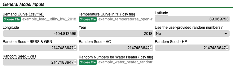
General Model Inputs
Demand Curve
The demand curve is the kW power generation from any existing utility-owned photovoltaic installations and/or existing chemical battery storage systems should be removed such that only the remaining (net) demand is portrayed. This must be formatted as a .csv file with a length of 8760 values representing the hourly demand (kW) for one entire year beginning on January 1.
Default: example_load_utility_kW_2018.csv (.csv file)
NOTE: All provided input data are assumed to begin on Jan 1. If the data correspond to a leap year, it is recommended to remove December 31 from the dataset. This preserves the extra day in February and allows the REopt model to run correctly (with 8760 total values).
An example of a valid .csv (shortened for brevity):
283416
275434
267785
263793
262463
262790
266827
269988
268817
...
318861
329671
320786
314194
306755
300396
291301
Temperature Curve
The temperature curve is the outdoor air temperature in degrees Fahrenheit corresponding to the utility’s service area and time corresponding to the Demand Curve. The format is a .csv file with a length of 8760 values representing the hourly temperature data in degrees Fahrenheit for the entire year.
Default: example_temperatures_open-meteo-denverCO-noheaders.csv (.csv file)
An example of a valid .csv (shortened for brevity):
4.6
3.3
2.7
2.8
3.6
4.4
2.8
5.1
5.2
6
...
17.9
17.9
18.4
17.4
16
11.4
10.8
10.7
10.6
10.6
10.4
Creating a Temperature Curve file
The easiest way to obtain a temperature curve .csv is by using the OpenMeteo temperature archive.
Begin by navigating to the OpenMeteo Historical Weather Data API and complete the following steps:
- Enter the approximate latitude and longitude of the utility or cooperative service area.
- The timezone should be the local time corresponding to the Demand Curve input data.
- Enter the Start Date (ex. 2018-01-01) and End Date (ex. 2018-12-31) of the year corresponding to the Demand Curve input data.
- Under the "Hourly Weather Variables" section, select “Temperature” only.
- Under "Settings" section, select Fahrenheit for the Temperature Unit. The other options may be left with the default values.
- Under the "API Response" section, reload the chart by pressing the “Reload Chart” button.
- Clicking the “Download CSV” button located under the API Response Chart that was just reloaded.
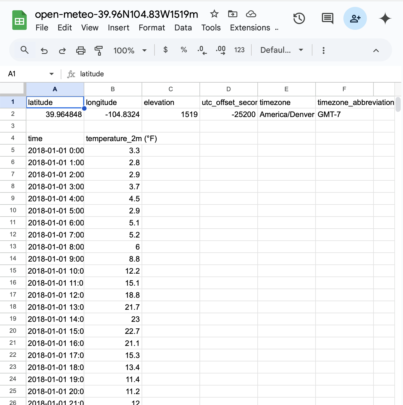
- Open the .csv file after downloading. It may be in your Downloads folder, or wherever your files go when they are downloaded. You want to be able to make changes and edit the file (e.g. the easiest way would be to open the file in Excel, Google Sheets, CryptPad Spreadsheet, OnlyOffice Spreadsheet, or some other spreadsheet program). The .csv file should look like this:
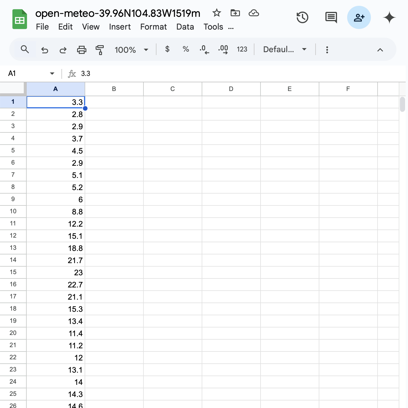
- Delete the header rows and the timestamp column. The .csv file should look like this when you upload it to derUtilityCost:
- Be sure that there are 8760 rows total. Save the file (e.g. if you’re using Google Sheets, go to File > Download > Comma Separated Values (.csv). Now you can upload the .csv file to the Temperature Curve input!
AFTER DOWNLOADING THE .CSV, YOU MUST EDIT THE .CSV FILE BY DOING THE FOLLOWING:
Latitude
The approximate latitude coordinate of the utility’s service area. The default case assumes the latitude for Brighton, CO.
Default: 39.986771 (decimal)
Longitude
The longitude coordinate of the utility’s approximate service area. The default case assumes the latitude for Brighton, CO.
Default: -104.812599 (decimal)
Year
The corresponding year for the Demand Curve input data.
Default: 2018 (int)
Use the user-provided random numbers?
Toggle to use either the user-provided random numbers or generate them automatically in the model. This input is used when the user wants to reproduce the same model run in the future.
If 'Yes' is selected, model will use all user-provided inputs for the Random Seeds (BESS & GEN, AC, HP, WH) and the Random Numbers for Water Heater (.csv) file.
If 'No' is selected, the model will generate all numbers needed and save them in the model outputs.
Default: No (Yes/No)
Random Seed - BESS & GEN
A deterministic random seed number for the HiGHS optimizer used for the BESS and GEN technologies. Must be a positive integer between 0 and 2147483647.
Default: 2147483647 (int)
Random Seed - AC
A deterministic random seed number for the PuLP optimizer used for the air conditioner technology. Must be a positive integer between 0 and 2147483647.
Default: 2147483647 (int)
Random Seed - WH
A deterministic random seed number for the PuLP optimizer used for the water heater technology. Must be a positive integer between 0 and 2147483647.
Default: 2147483647 (int)
Random Seed - HP
A deterministic random seed number for the PuLP optimizer used for the heat pump technology. Must be a positive integer between 0 and 2147483647.
Default: 2147483647 (int)
Random Numbers for Water Heater
A file with random numbers that will help determine the water heater's water draw in gallons per minute. If the Use the user-provided random numbers? input is set to 'Yes', the model will use the provided file. If 'No', the model will generate and save a water_heater_random_numbers.csv file in the ouput files, which the user can re-upload here.
Default: example_water_heater_random_numbers.csv (.csv file)
Example file:
16.0,-5.0,0.2092334309280378
16.0,-11.0,0.2745899659231128
7.0,-14.0,0.5489484822693608
1.0,-5.0,0.09139400225934302
16.0,-3.0,0.10289385741323365
4.0,-8.0,0.22365900110938863
18.0,-9.0,0.6779007018291736
15.0,-8.0,0.8535451643255744
9.0,-10.0,0.1500305671738359
0.0,-14.0,0.15522609801142717
7.0,-4.0,0.6510939156408193
10.0,-14.0,0.6588429262558114
7.0,-12.0,0.37739650648188483
9.0,-8.0,0.06891053041774076
1.0,-12.0,0.9234201707499036
18.0,-9.0,0.5719325012746554
10.0,-14.0,0.04001062962865709
6.0,-10.0,0.5998936023082809
0.0,-11.0,0.5138174552600452
12.0,-8.0,0.5616127576754277
14.0,-11.0,0.6225784880932328
10.0,-6.0,0.6467697799429435
11.0,-12.0,0.9760783132839952
12.0,-1.0,0.9197215740009584
13.0,-10.0,0.14526456212839922
9.0,-8.0,0.6786767390786106
7.0,-9.0,0.9636663619478575
0.0,-9.0,0.44224156114764224
3.0,-3.0,0.10156915120952226
2.0,-3.0,0.48449884928990516
0.0,-9.0,0.2282449787151043
14.0,-8.0,0.7371555612663239
13.0,-9.0,0.30349532304568594
6.0,-11.0,0.5328064314629861
15.0,0.0,0.5942292068693534
8.0,-4.0,0.8254863973602222
12.0,0.0,0.6099561570281333
13.0,-12.0,0.8241152639145998
12.0,-12.0,0.8553491706622669
3.0,-1.0,0.4908047336002531
17.0,-11.0,0.18887860946325252
5.0,-6.0,0.39583115105876754
8.0,0.0,0.6557597208727626
5.0,-9.0,0.7281912887423867
18.0,-8.0,0.4467830583804442
7.0,-7.0,0.04741084173487231
9.0,-10.0,0.009101483074423378
14.0,0.0,0.4397843601619892
9.0,-10.0,0.6117952886582574
6.0,-14.0,0.18089021913033387
For instructions on how to generate a water_heater_random_numbers.csv file and reproduce the same water heater results between runs, see How to Reproduce Model Results.
Financial Inputs
This section contains the financial inputs for the model.
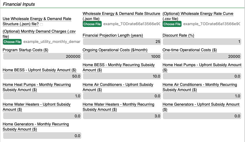
Use Wholesale Energy & Demand Rate Structure (.json) file?
This input toggles the choice between using the Wholesale Energy & Demand Structure (.json) OR the two optional CSV inputs: (Optional) Wholesale Energy Rate Curve (.csv) file and the (Optional) Monthly Demand Charges (.csv) file to upload the wholesale tariff information.
If the checkbox is selected, the model will use the user-provided Wholesale Energy & Demand Structure (.json) file. This file is best suited for tiered energy rate structures and hourly demand information (NOTE: if the user has a monthly demand rate structure, then it is recommended to uncheck this box and use the two optional CSV inputs (Optional) Wholesale Energy Rate Curve (.csv) and (Optional) Monthly Demand Charges (.csv)).
If the checkbox is not selected, the model will instead use the two CSV inputs (Optional) Wholesale Energy Rate Curve (.csv) and (Optional) Monthly Demand Charges (.csv) file.. These are separate inputs, allowing the user to upload an hourly energy rate structure and a monthly demand rate structure.
Default: Unchecked (Checked/Unchecked). The default uses the (Optional) Wholesale Energy Rate Curve (.csv) and (Optional) Monthly Demand Charges (.csv) files.
Wholesale Energy & Demand Rate Structure
This is a .json file describing the wholesale energy and demand rate structure that utility pays to their G&T or other provider for their energy. This input allows a utility to upload a custom rate structure if the URDB Label is not known or is incorrect. An example of a valid .json file:
Default: example_TODrate66a13566e90ecdb7d40581d2.json (.json file)
{"energyweekdayschedule":[[1,1,1,1,1,1,1,1,1,1,1,1,1,1,2,2,2,2,2,2,2,2,1,1],[1,1,1,1,1,1,1,1,1,1,1,1,1,1,2,2,2,2,2,2,2,2,1,1],[1,1,1,1,1,1,1,1,1,1,1,1,1,1,2,2,2,2,2,2,2,2,1,1],[1,1,1,1,1,1,1,1,1,1,1,1,1,1,2,2,2,2,2,2,2,2,1,1],[1,1,1,1,1,1,1,1,1,1,1,1,1,1,2,2,2,2,2,2,2,2,1,1],[1,1,1,1,1,1,1,1,1,1,1,1,1,1,2,2,2,2,2,2,2,2,1,1],[1,1,1,1,1,1,1,1,1,1,1,1,1,1,2,2,2,2,2,2,2,2,1,1],[1,1,1,1,1,1,1,1,1,1,1,1,1,1,2,2,2,2,2,2,2,2,1,1],[1,1,1,1,1,1,1,1,1,1,1,1,1,1,2,2,2,2,2,2,2,2,1,1],[1,1,1,1,1,1,1,1,1,1,1,1,1,1,2,2,2,2,2,2,2,2,1,1],[1,1,1,1,1,1,1,1,1,1,1,1,1,1,2,2,2,2,2,2,2,2,1,1],[1,1,1,1,1,1,1,1,1,1,1,1,1,1,2,2,2,2,2,2,2,2,1,1]],"energyweekendschedule":[[1,1,1,1,1,1,1,1,1,1,1,1,1,1,2,2,2,2,2,2,2,2,1,1],[1,1,1,1,1,1,1,1,1,1,1,1,1,1,2,2,2,2,2,2,2,2,1,1],[1,1,1,1,1,1,1,1,1,1,1,1,1,1,2,2,2,2,2,2,2,2,1,1],[1,1,1,1,1,1,1,1,1,1,1,1,1,1,2,2,2,2,2,2,2,2,1,1],[1,1,1,1,1,1,1,1,1,1,1,1,1,1,2,2,2,2,2,2,2,2,1,1],[1,1,1,1,1,1,1,1,1,1,1,1,1,1,2,2,2,2,2,2,2,2,1,1],[1,1,1,1,1,1,1,1,1,1,1,1,1,1,2,2,2,2,2,2,2,2,1,1],[1,1,1,1,1,1,1,1,1,1,1,1,1,1,2,2,2,2,2,2,2,2,1,1],[1,1,1,1,1,1,1,1,1,1,1,1,1,1,2,2,2,2,2,2,2,2,1,1],[1,1,1,1,1,1,1,1,1,1,1,1,1,1,2,2,2,2,2,2,2,2,1,1],[1,1,1,1,1,1,1,1,1,1,1,1,1,1,2,2,2,2,2,2,2,2,1,1],[1,1,1,1,1,1,1,1,1,1,1,1,1,1,2,2,2,2,2,2,2,2,1,1]],"energyratestructure":[[{"rate":0,"unit":"kWh"}],[{"rate":0.06,"unit":"kWh"}],[{"rate":0.1525,"unit":"kWh"}]],"demandratestructure":[[{"rate":0,"unit":"kW"}],[{"rate":4,"unit":"kW"}]],"demandweekdayschedule":[[1,1,1,1,1,1,1,1,1,1,1,1,1,1,1,1,1,1,1,1,1,1,1,1],[1,1,1,1,1,1,1,1,1,1,1,1,1,1,1,1,1,1,1,1,1,1,1,1],[1,1,1,1,1,1,1,1,1,1,1,1,1,1,1,1,1,1,1,1,1,1,1,1],[1,1,1,1,1,1,1,1,1,1,1,1,1,1,1,1,1,1,1,1,1,1,1,1],[1,1,1,1,1,1,1,1,1,1,1,1,1,1,1,1,1,1,1,1,1,1,1,1],[1,1,1,1,1,1,1,1,1,1,1,1,1,1,1,1,1,1,1,1,1,1,1,1],[1,1,1,1,1,1,1,1,1,1,1,1,1,1,1,1,1,1,1,1,1,1,1,1],[1,1,1,1,1,1,1,1,1,1,1,1,1,1,1,1,1,1,1,1,1,1,1,1],[1,1,1,1,1,1,1,1,1,1,1,1,1,1,1,1,1,1,1,1,1,1,1,1],[1,1,1,1,1,1,1,1,1,1,1,1,1,1,1,1,1,1,1,1,1,1,1,1],[1,1,1,1,1,1,1,1,1,1,1,1,1,1,1,1,1,1,1,1,1,1,1,1],[1,1,1,1,1,1,1,1,1,1,1,1,1,1,1,1,1,1,1,1,1,1,1,1]],"demandweekendschedule":[[1,1,1,1,1,1,1,1,1,1,1,1,1,1,1,1,1,1,1,1,1,1,1,1],[1,1,1,1,1,1,1,1,1,1,1,1,1,1,1,1,1,1,1,1,1,1,1,1],[1,1,1,1,1,1,1,1,1,1,1,1,1,1,1,1,1,1,1,1,1,1,1,1],[1,1,1,1,1,1,1,1,1,1,1,1,1,1,1,1,1,1,1,1,1,1,1,1],[1,1,1,1,1,1,1,1,1,1,1,1,1,1,1,1,1,1,1,1,1,1,1,1],[1,1,1,1,1,1,1,1,1,1,1,1,1,1,1,1,1,1,1,1,1,1,1,1],[1,1,1,1,1,1,1,1,1,1,1,1,1,1,1,1,1,1,1,1,1,1,1,1],[1,1,1,1,1,1,1,1,1,1,1,1,1,1,1,1,1,1,1,1,1,1,1,1],[1,1,1,1,1,1,1,1,1,1,1,1,1,1,1,1,1,1,1,1,1,1,1,1],[1,1,1,1,1,1,1,1,1,1,1,1,1,1,1,1,1,1,1,1,1,1,1,1],[1,1,1,1,1,1,1,1,1,1,1,1,1,1,1,1,1,1,1,1,1,1,1,1],[1,1,1,1,1,1,1,1,1,1,1,1,1,1,1,1,1,1,1,1,1,1,1,1]]}
The example above was created using the REopt Web Tool custom electric rate tariff generator following their instructions: https://github.com/NREL/REopt-Analysis-Scripts/wiki/5.-Custom-Electric-Rates. The rate structure information was based on a Colorado utility's Time of Day residential rate structure found at https://apps.openei.org/USURDB/rate/view/66a13566e90ecdb7d40581d2#3__Energy.
Although the REopt Web Tool provides options to include more information (e.g. Fixed monthly charge, facility demand charge), the derUtilityCost model currently does not handle that information. If monthly demand charges are desired, then it's suggested to use the optional Monthly Demand Charges (.csv) input along with the optional Wholesale Energy Rate Curve (.csv) input, and un-selecting the Use Wholesale Energy & Demand Rate Structure (.json) file? input to allow these optional inputs to be used.
(Optional) Wholesale Energy Rate Curve
A .csv file containing 8760 rows representing the hourly \$/kWh rate that the utility or cooperative pays to the wholesale energy supplier.
Default: example_TODrate66a13566e90ecdb7d40581d2.csv (.csv file)
Example of a valid .csv (shortened for brevity):
0.0600
0.0600
0.0600
0.0600
0.0600
0.0600
0.0600
0.0600
0.0600
0.0600
...
0.0600
0.1525
0.1525
0.1525
0.1525
0.1525
0.1525
0.1525
0.1525
0.0600
0.0600
(Optional) Monthly Demand Charges
The monthly demand charges (\$/kW) that the utility pays their G&T provider for the entire Year. The expected format is a .csv file containing 12 elements corresponding to each month. For example:
Default: example_utility_monthly_demand_charges.csv (.csv)
50
50
50
50
50
50
50
50
50
50
50
50
This file represents \$50/hr demand charge for all 12 months.
Financial Projection Length
The number of years to project out estimated financial savings. Must be between 1 and 75 years. Note that the financial analysis only takes into account the first year (since only a one year demand curve is provided) and project those financial findings out for all subsequent years.
Default: 25 (int, unit: years)
Discount Rate
The discount rate is used to devalue future incomes in the financial analysis when calculating the Net Present Value. Income received now is generally more valuable than income received later.
Default: 1 (int, unit: %)
Program Startup Costs
The total costs for the utility to start the DER program.
Default: 200000 (int/decimal, unit: \$)
Ongoing Operational Costs
The total monthly costs to the utility for all operational costs (e.g. API calls per month).
Default: 1000 (int/decimal, unit: \$/month).
One-time Operational Costs
The total one-time costs to the utility for all operational costs (e.g. contracted agreements for DER device usage, etc.).
Default: 20000 (int/decimal, unit: \$)
Home BESS - Upfront Subsidy Amount
The one-time subsidy amount paid to the member-consumer for enrolling their BESS in the DER-sharing program.
Default: 50.0 (int/decimal, unit: \$)
Home BESS - Monthly Recurring Subsidy Amount
The monthly subsidy paid to the member-consumer for continuous monthly participation in the DER-sharing program.
Default: 10.0 (int/decimal, unit: \$)
Home Heat Pump - Upfront Subsidy Amount
The one-time subsidy amount paid to the member-consumer for enrolling their Heat Pump in the DER-sharing program.
Default: 0.0 (int/decimal, unit: \$)
Home Heat Pump - Monthly Recurring Subsidy Amount
The monthly subsidy paid to the member-consumer for continuous monthly participation in the DER-sharing program.
Default: 1.0 (int/decimal, unit: \$)
Home Air Conditioner - Upfront Subsidy Amount
The one-time subsidy amount paid to the member-consumer for enrolling their Air Conditioner in the DER-sharing program.
Default: 0.0 (int/decimal, unit: \$)
Home Air Conditioner - Monthly Recurring Subsidy Amount
The monthly subsidy paid to the member-consumer for continuous monthly participation in the DER-sharing program.
Default: 1.0 (int/decimal, unit: \$)
Home Water Heater - Upfront Subsidy Amount
The one-time subsidy amount paid to the member-consumer for enrolling their Water Heater in the DER-sharing program.
Default: 0.0 (int/decimal, unit: \$)
Home Water Heater - Monthly Recurring Subsidy Amount
The monthly subsidy paid to the member-consumer for continuous monthly participation in the DER-sharing program.
Default: 3.0 (int/decimal, unit: \$)
Home Generators - Upfront Subsidy Amount
The one-time subsidy amount paid to the member-consumer for enrolling their fossil fuel generator in the DER-sharing program.
Default: 0.0 (int/decimal, unit: \$)
Home Generators - Monthly Recurring Subsidy Amount
The monthly subsidy paid to the member-consumer for continuous monthly participation in the DER-sharing program.
Default: 0.0 (int/decimal, unit: \$)
Home Fossil Fuel Device Inputs
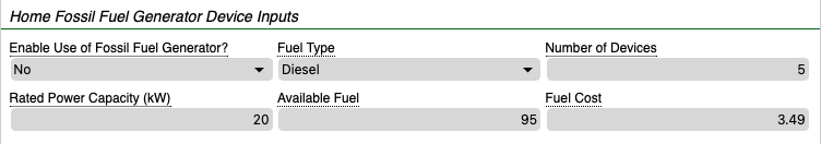
Enable Use of Fossil Fuel Generator?
This toggle enables or disables the fossil fuel generator technology in the analysis. If "Yes" is selected, the model will include fossil fuel generators in the analysis. If "No" is selected, the model will not include fossil fuel generators in the analysis.
Default: No (Yes/No)
Fuel Type
The type of fossil fuel used for all generators. Each fuel type has different default inputs for the Fuel Cost and Available Fuel inputs according to the table below.
Default: Diesel (Natural Gas/Propane/Diesel/Gasoline)
| Fuel Type | Efficiency | Fuel Cost[1] | Available Fuel |
|---|---|---|---|
| Natural Gas | 30\%[4] | \$0.00386/cu.ft. | 1000 cu.ft. |
| Propane | 25\%[2][4] | \$2.70/gallon | 1000 gallons |
| Diesel | 35\%[3][4] | \$3.80/gallon | 1000 gallons |
| Gasoline | 25\%[3][4] | \$3.17/gallon | 1000 gallons |
| --- |
Number of Home Fossil Fuel Generators
Total number of home fossil fuel generators to include in the model.
Default: 5 (int)
Rated Power Capacity
The average capacity size (kW) of each home fossil fuel generator. The default value is based on a Generac 20 kW diesel generator.
Default: 20 (int, unit: kW)
Available Fuel
The maximum amount of generator fuel available per device. The default value is based on a Generac 20 kW diesel model with a fuel tank capacity of 95 gallons. This input will change if a different fuel type is selected (see table above).
Default: 95 (int, unit: gallons)
Fuel Cost
The cost in USD per gallon (or cu.ft. in the case of natural gas) of fuel used for the generator. This input will change if a different fuel type is selected (see table above).
Default: 3.49 (decimal, unit: \$/gal)
Chemical Energy Storage Device Inputs
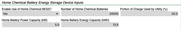
Enable Use of Home Chemical BESS?
Toggle to enable or disable the use of home chemical battery energy storage system in the model. If Yes, the model will include Home Chemical BESS in the analysis. If No, the model will not include any.
Default: Yes (Yes/No)
Number of Home Chemical Batteries
Total number of residential chemical batteries to model.
Default: 20000 (int)
Portion of Charge Used by Utility
The maximum percentage of full charge per home chemical BESS that is available for the utility to use at any time.
Default: 20.0 (int, unit: %)
Home Battery Power Capacity
The battery power capacity in kW for each individual battery enrolled by a member-consumer. The default value corresponds to a Tesla Powerwall battery.
Default: 5.0 (decimal, unit: kW)
Home Battery Energy Capacity
The battery energy capacity in kWh for each individual battery enrolled by a member-consumer. The default value corresponds to a Tesla Powerwall battery.
Default:13.5 (decimal, unit: kWh)
Home Air Conditioner Device Inputs
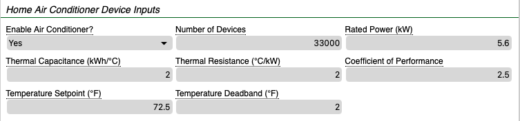
Enable Air Conditioner?
If Yes, the model will run with a home central air conditioner. If No, the model will not run with a home air conditioner.
Default: Yes (Yes/No)
Number of Air Conditioner Devices
Total number of home air conditioner devices to simulate.
Default: 33000 (int)
Rated Power
Maximum input power of the air conditioner. Must be a positive rational number between 0.1 and 7.2. The default value 5.6 represents a central AC system. For in-window units, use a value of around 0.5.
Default: 5.6 (decimal, unit: kW)
Thermal Capacitance
Thermal capacitance of the air conditioner. Must be between 0.2 and 2.5 with exactly one decimal digit.
Default: 2.0 (decimal, unit: kWh/°C)
Thermal Resistance
Thermal resistance of the air conditioner. Must be between 1.5 and 140.
Default: 2.0 (decimal, unit: °C/kW)
Coefficient of Performance
Coefficient of performance for the air conditioner. Must be between 1 and 3.5.
Default:2.5 (decimal)
Temperature Setpoint
Target temperature for the air conditioner, set at the thermostat. Must be between 35.06 and 129.2.
Default: 72.5 (decimal, unit: °F)
Temperature Deadband
Deadband around the setpoint temperature to alleviate temperature swings. Must be between 0.225 and 3.6.
Default: 2.0 (decimal, unit: °F)
Home Heat Pump Device Inputs
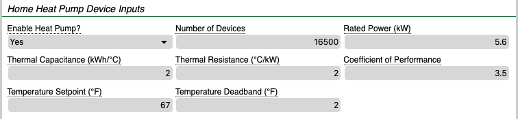
Enable Heat Pump?
This toggle enables or disables the heat pump technology in the analysis. If 'Yes', the model will run with a home air-source heat pump. If 'No', the model will not run with a heat pump.
Default: Yes (Yes/No)
Number of Heat Pump Devices
Total number of home heat pump devices to simulate.
Default: 16500
Rated Power
Maximum input power of the heat pump. Must be a positive rational number between 0.1 and 7.2.
Default: 5.6 (decimal, unit: kW)
Thermal Capacitance
Thermal capacitance of the heat pump. Must be between 0.2 and 2.5 with exactly one decimal digit.
Default: 2.0 (decimal, unit: kWh/°C)
Thermal Resistance
Thermal resistance of the heat pump. Must be between 1.5 and 140.
Default: 2.0 (decimal, unit: °C/kW)
Coefficient of Performance
Coefficient of performance for the heat pump. Must be between 1 and 3.5
Default: 3.5 (decimal)
Temperature Setpoint
Target temperature for the heat pump, set at the thermostat. Must be between 35.06 and 129.2.
Default: 67.0 (decimal, unit: °F)
Temperature Deadband
Deadband around the setpoint; avoids excessive cycling of heat pump. Must be between 0.225 and 3.6.
Default: 2.0 (decimal, unit: °F)
Home Water Heater Device Inputs
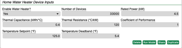
Enable Water Heater?
This toggle enables or disables the water heater technology in the analysis. If 'Yes', model will run with home water heaters. If 'No', model will not use any water heaters.
Default: Yes (Yes/No)
Number of Water Heater Devices
Total number of home water heater devices to simulate.
Default: 33000 (int)
Rated Power
Maximum input power of the water heater. Must be a positive rational number between 0.1 and 7.2.
Default: 4.5 (decimal, unit: kW)
Thermal Capacitance
Thermal capacitance of the water tank. Must be between 0.2 and 2.5 with exactly one decimal digit.
Default: 0.4 (decimal, unit: kWh/°C).
Thermal Resistance
Thermal resistance of the water tank. Must be between 1.5 and 140.
Default: 120.0 (decimal, unit: °C/kW)
Coefficient of Performance
Coefficient of performance for the water heater. Must be between 1 and 3.5
Default: 1.0 (int)
Temperature Setpoint
Target temperature for the tank, set at the thermostat. Must be between 35.06 and 129.2.
Default: 125.0 (decimal, unit: °F)
Temperature Deadband
Deadband around the setpoint temperature to alleviate swings in temperature. Must be between 0.225 and 5.4.
Default: 5.4 (decimal, unit: °F)
Model Results
The chosen color schemes used for these plots are based on the following guide for color-blind friendly color schemes: 2022 NCEAS Science Communication Resource Corner by Alexandra Phillips
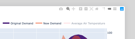
Plot: Impact to Demand
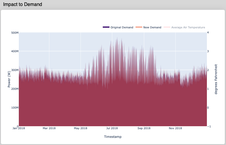 This plot shows the Original Demand (demand curve without DER) and the New Demand (demand curve with DER). The Outdoor Air Temperature variable can be toggled on/off by clicking on the name.
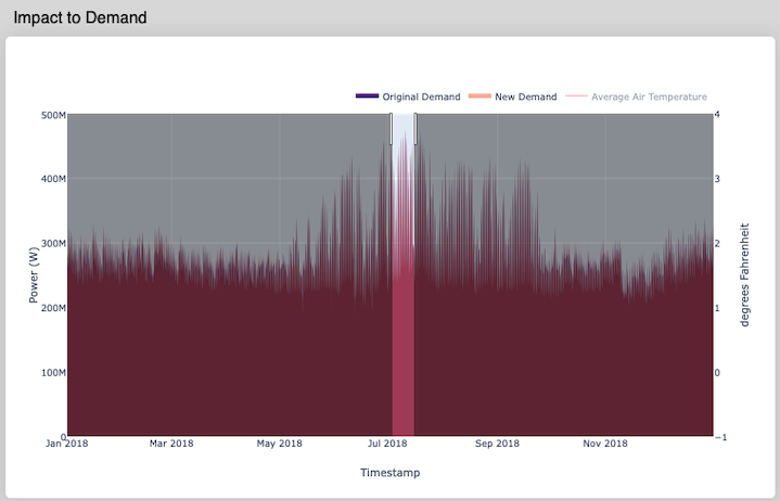 To zoom in, drag and hold the mouse cursor across the desired timeframe. The plot will zoom in when you let go of the cursor.
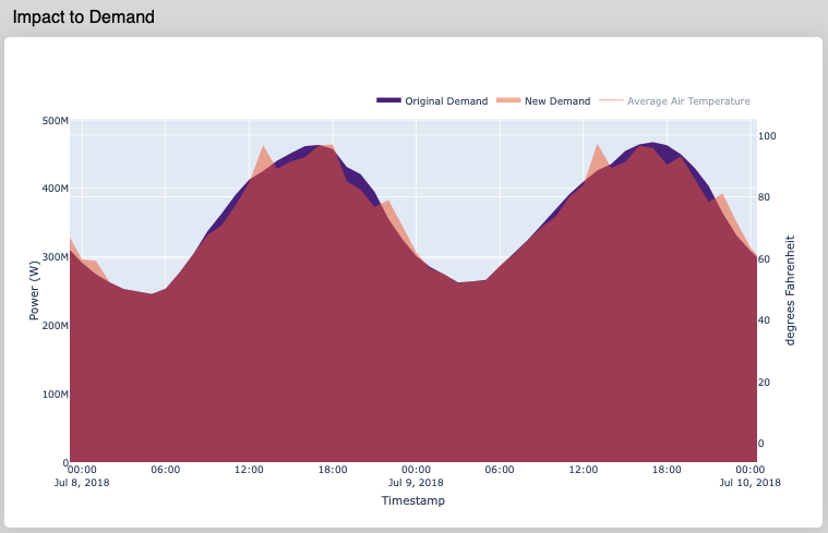 This is a zoomed-in plot showing a two day timescale.
To reset the window or zoom all the way back out, hover the mouse over the top right corner of the plot and select "Reset Axes".
To pan around the plot, select the "Pan" icon and then drag the plot around. If you are zoomed in and want to shift the plot left or right, hold down the COMMAND key (on MacOS) while dragging the plot left or right.
Plot: DER Serving Load Overview
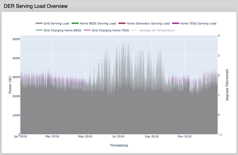 This plot shows the breakdown of all DER serving the load and charging from the grid. All thermal technologies are aggregated into the Thermal Energy Storage System (TESS) variable. Like the Impact to Demand Plot, this plot can be zoomed into if desired.
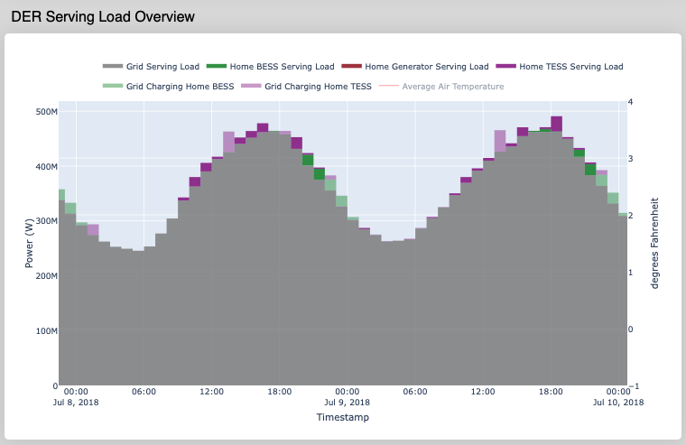 This shows a zoom-in on a two-day window.
Plot: Thermal DER Serving Load Overview

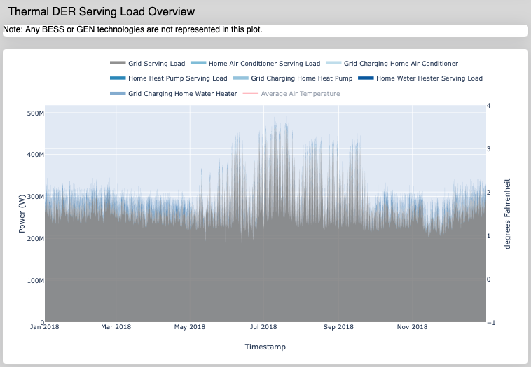 This plot shows a more detailed breakdown of the thermal DER technologies (Water Heater, Air Conditioner, and Heat Pump) that serve the utility’s load throughout the year. Note that this plot does not show the BESS or GEN technologies, it is purely for looking at the thermal technologies. The Grid Serving Load is still present in this plot, however (see the previous DER Serving Load Overview plot).
This detailed view of the thermal technologies allows a utility to analyze the behavior for a specific thermal technology during a specific hour, day, or month of the year.
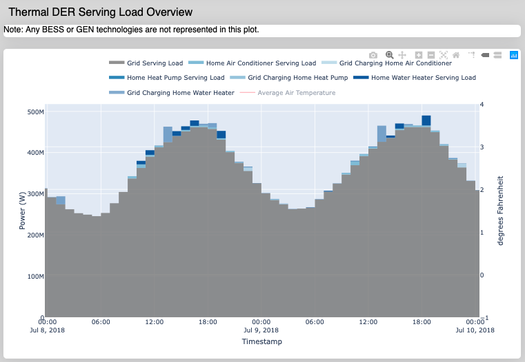 The plot is zoomed into a two-day timescale here.
Prioritization of Water Heater, Air Conditioner, and Heat Pump
Each type of thermal technology (WH, AC, HP) is calculated independently from the others because of the constraints of the vbatDispatch model. A result of this decoupling is instances of two or more technologies charging at the same time, which can create a larger peak demand (and thus larger expense) for the utility. To address this, a thermal DER prioritization plan was introduced into the code that prevents multiple devices from charging simultaneously. The thermal technologies are prioritized in the following order:
Water Heater > Air Conditioner > Heat Pump
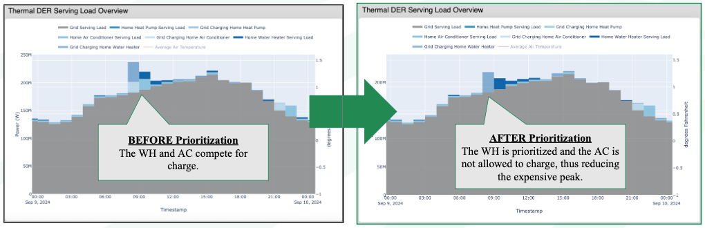
When two or more technologies compete for charge at the same time, only the highest priority technology is allowed to charge and discharge. In the case of the figures shown above, the WH and AC competed for charge time before the prioritization code was implemented. After the prioritization, only the WH is allowed to charge (and thus the AC does not charge or discharge). Be aware of the bias towards Water Heaters in the results of your model run.
How to Reproduce Model Results
It is useful to investigate how changing certain input parameters affects the model results. To do this, one would need to reproduce the same exact model with only the user changes reflected. Normally, there is some variation in the model results due to the optimization methods used inside the model. Specifically, this is due to changes in the random seed for every model run in addition to an optimality tolerance parameter in the optimizers (i.e. HiGHS and CBC) used by REopt and vbatDispatch. The Water Heater code additionally uses random numbers to generate a water draw rate.
To reproduce the results of a model run:
- If you have a completed run already, skip this step. If you do not have a model run you'd like to reproduce, simply run a model with any desired inputs and/or run the model with `Use the user provided random numbers?` input to 'No'.
- In the completed model run that you'd like to reproduce the results of, navigate to the Raw Input and Output Files section at the bottom of the model screen.
- Save the `water_heater_random_numbers.csv` file. On MacOS, this is done by right-clicking the file and selecting "Download Linked File As..."
- Also in the Raw Input and Output files, locate the random_seeds.csv file. Contained in that file for each technology enabled is a random seed number between 0 and 2147483647. Record or note the values for each technology.
- Go back up to the end of the Model Inputs and Duplicate the model using the green button. Give it a new name.
- In the duplicated model, input the corresponding random seed numbers into the random seed inputs in the General Model Inputs section (i.e. Random Seed - BESS \& GEN, Random Seed - AC, etc.) and upload the water_heater_random_numbers.csv file you saved earlier.
- Ensure that the `Use the User-provided random numbers?` input is set to `Yes`.
- For the `Use the user-provided random numbers?` input, select `Yes`.
- Ensure that all model inputs are the same as your previous model run. Do not change any inputs yet.
- Run the duplicated model.
- Compare the output plot results with the previous desired model. I like to look at the Cash Flow Projection Plot and see if the Utility Savings is identical. If not, carefully review that all steps were done correctly.
- After confirming that the results can be reproduced, you can make changes to the inputs in your duplicated model, run again, and continue your analysis!
Plot: Home Thermal Battery Power Profile
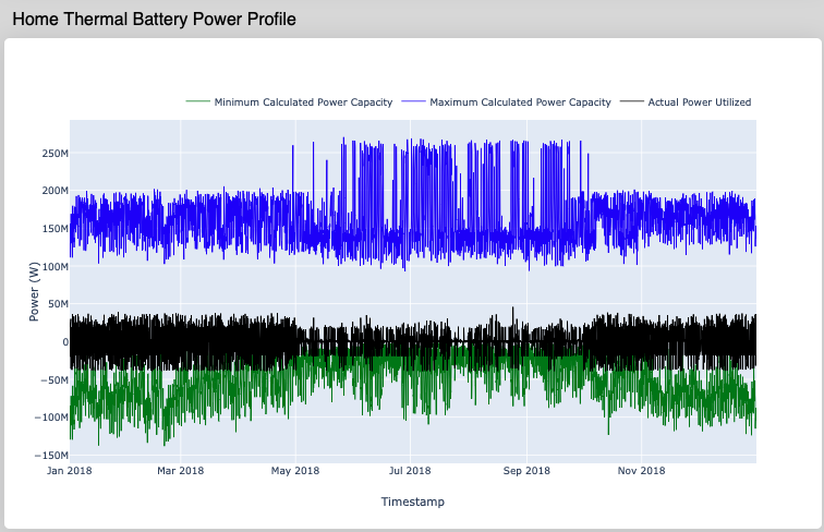 This plot shows the minimum and maximum calculated power capacity and the Actual Power Utilized for all of the thermal technologies combined. This is useful for diagnosing the behavior of the thermal technologies and/or the underlying vbatDispatch model used to simulate them.
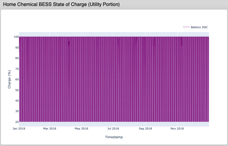
Plot: Home Chemical BESS State of Charge (Utility Portion)
 This plot shows the state of charge of all chemical batteries in the analysis. 100% here means the maximum charge of the battery allowed to the utility. If the
 Portion of Charge Used by Utility (%) input is 20\%, then 100% in this plot would correspond to the full 20\% of every chemical battery's energy capacity (kWh) allowed for utility use.
Table: Monthly Cost Comparison
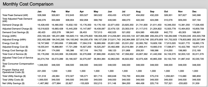 This plot shows a detailed monthly overview of all the energy, demand, and financial variables. Below is a detailed explanation of each variable in this plot.
Total Peak Demand (kW)
This is the total peak demand (kW) for each month. If the Use Wholesale Energy & Demand Rate Structure (.json) file? is selected and the user provides demand rate structure information in that .json file, the Total Peak Demand (kW) is the sum of all the corresponding kW for the maximum dollar amount (peak kW x rate \$/kW) in each rate period window during that month.
For example, if the demandratestructure in the .json file has rates of 0, 0.01, 1, this corresponds Rate Periods numbered 0, 1, 2. For the month of January, let's say Rate Period 1 is applied every day from 12am-12pm, and Rate Period 2 is applied every day from 12pm - 12am. Within each rate period, the hourly kW in January from the Demand Curve is multiplied by the demand rate for that rate period (e.g. at 1am on Jan 1 if the kW is 2.4 kW, then the demand charge dollar amount is equal to 2.4 kW x \$0.01/kW = \$0.024). Then, the corresponding kW of the maximum dollar amount between all the demand charge dollar amounts in Period 1 on Jan 1 is added to the Total Peak Demand (kW), and the same is done for Period 2 on Jan 1, Period 1 on Jan 2, Period 2 on Jan 2, and so on.
Total Adjusted Peak Demand (kW):
This is similar to the Total Peak Demand (kW) but performed e for the demand curve that has been adjusted by the DERs discharging and charging.
Demand Charge:
If the Use Wholesale Energy & Demand Rate Structure (.json) file? is selected and the user provides demand rate structure information in that .json file, then the demand charge is calculated as the total monthly peak demand cost (\$). If the demand rate tariff is a flat rate \$/kW for each month, this is simply the maximum dollar amount for the month when each hour's demand (kW) is multiplied by the \$/kW of that month. If the demand rate tariff is more complex (e.g. a weekday window of 2-8pm is charged at some \$/kW rate, whereas a weekend window could be 5-10pm at a different \$/kW rate, and so on), then the maximum peak dollar amount (\$) is the sum of all the maximum peak dollar amounts in each rate period window of that month (i.e. in each 2-8pm window there is a maximum \$ amount found by multiplying each hour kW by the corresponding \$/kW rate and taking the maximum \$. All maximum \$ amounts in each 2-8pm window in that month is added together to get the total monthly \$ for that window. If there are any other windows such as the 5-10pm weekend rate example, those are calculated similarly and added together for the month. All total maximum \$ for all rate period windows are added together to give the total monthly demand charge).
If the Use Wholesale Energy & Demand Rate Structure (.json) file? is NOT selected and the user provides demand rate structure information in the (Optional) Monthly Demand Charges (.csv) file, then the demand charge is calculated the same as described above using the rate information in the (Optional) Monthly Demand Charges (.csv) file.
Adjusted Demand Charge:
Similar to the Demand Charge calculation, but performed for the demand curve that has been adjusted by DERs discharging and charging.
Demand Cost Savings:
For each month of the year, this shows the demand savings given by Demand Charge - Adjusted Demand Charge.
Energy (kWh):
For each month of the year, this shows the sum total kWh of the Demand Curve.
Adjusted Energy (kWh):
The monthly Energy that includes the adjustments made by all DERs discharging and charging.
Energy Cost (\$):
For each month of the year, this is the sum total of Energy multiplied by each corresponding hourly energy tariff \$/kWh.
Adjusted Energy Cost (\$):
The adjusted energy cost is similar to Energy Cost, but it uses the demand curve that has been adjusted by all DERs discharging and charging. For each month, the adjusted energy cost is the sum total of the Adjusted Energy multiplied by the energy tariff (\$/kWh) for each corresponding hour.
Energy Cost Savings (\$):
This is calculated by taking the difference between the Energy Cost and Adjusted Energy Cost: Energy Cost - Adjusted Energy Cost.
Total Cost of Service (\$):
This is calculated by adding Energy Cost and Demand Charge: Energy Cost + Demand Charge.
Adjusted Total Cost of Service (\$):
This is calculated by adding Adjusted Energy Cost and Adjusted Demand Charge: Adjusted Energy Cost and Adjusted Demand Charge.
Total Consumer Compensation (\$):
This is the sum total dollar amount paid to the member-consumer for all subsidies.
Program Startup and Operational Costs (\$):
This is a fixed cost representing any one-time startup or operational costs the utility pays to begin the DER sharing program.
Total Utility Savings (\$):
This is the total savings for the utility given by Energy Cost Savings + Demand Cost Savings
Total Utility Costs (\$):
For each month, this is the total costs for the utility given by Program Startup and Operational Costs + subsidies paid to consumer.
Net Utility Savings (\$):
This is the net savings for the utility given by Total Utility Savings - Total Utility Costs.
Plot: Cash Flow Projection
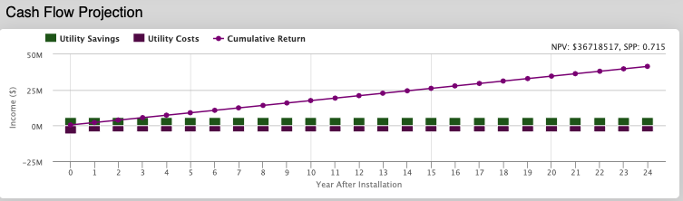 This plot shows the yearly cash flow projection based only on the results from year 1 (see Monthly Cost Comparison table for year 1 values). The
 Utility Savings is the sum of the monthly Total Utility Savings values in the Monthly Cost Comparison chart, and the Utility Costs are similarly the sum of the monthly Total Utility Costs in the Monthly Cost Comparison chart. The Cumulative Return series is the cumulative sum of the Net Utility Savings cash flow.
Simply click on the variable names to toggle them on/off.
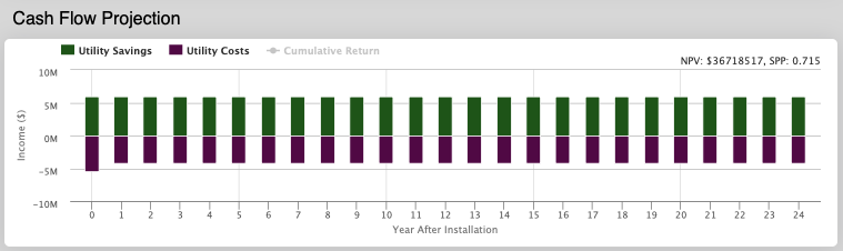 Here the
 Cumulative Return is toggled OFF.
Note the Net Present Value (NPV) and Simple Payback Period (SPP) are shown in the top right corner of this plot.
Net Present Value
The NPV is the value of all future cash flows over an investment’s lifetime, discounted to the present. This is represented by the equation:
$\displaystyle\sum_{t=0}^{M-1} \frac{values_t}{(1+rate)^t}$ [5]
Where rate is the discount rate given as user input in the General Model Inputs, and values are the projected cash flows = (Utility Savings – Utility Costs)$_t$ for each year, $t$, up to a total projection length of $M$ years.
Utility Savings = all DER kW Demand Savings (\$) + all DER kWh Consumption Savings (\$)
Utility Costs = startup costs (\$) + all operational costs (\$) + all subsidies (\$)
Simple Payback Period
The SPP is the number of years it takes to recover all initial costs based on the first year’s cash flows. It is represented by the following equation:
$\frac{\rm{Initial \ Investment}}{\rm{Utility \ Savings}-\rm{Utility \ Costs}}$
Where Initial Investment = startup costs (\$) + one-time operational costs (\$) + one-time subsidies (\$)
Utility Savings = all DER Demand (kW) Savings in Year 1 + all DER Consumption (kWh) Savings in Year 1
Utility Costs = ongoing operational costs in Year 1 + all DER ongoing subsidies in Year 1
Plot: Savings Breakdown Per Technology
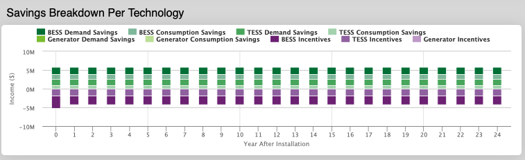 This plot shows the yearly savings and incentives breakdown for the BESS, TESS, and GEN technologies (if enabled).
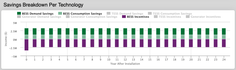 This shows only the BESS Savings and BESS Incentives toggled on, for example.
This plot is useful for technology-specific insights for evaluating the overall benefit of individual DER. TESS here is an aggregate of all thermal technologies (i.e. WH+AC+HP).
The incentives represent the subsidy amounts for each technology. The savings are broken up into a Demand (kW) Savings and a Consumption (kWh) savings for each DER.
Plot: Savings Breakdown of Thermal Technologies
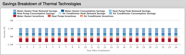 This plot shows the yearly savings and incentives breakdown of only the TESS technologies: Water Heater, Heat Pump, and Air Conditioner, if enabled.
This is useful for evaluating the individual thermal DER.
Raw Input and Output Files
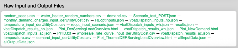 At the very end of the model outputs is a collection of all raw inputs and outputs for that model run:
- random_seeds.csv
- water_heater_random_numbers.csv
- demand.csv
- Scenario_test_POST.json
- monthly_demand_charges_input_derUtilityCost.csv
- REoptInputs.json
- vbatDispatch_inputs_hp.json
- temperature_input_derUtilityCost.csv
- reopt_input_scenario.json
- vbatDispatch_inputs_wh.json
- results.json
- vbatDispatch_results_hp.json
- Plot_DerServingLoadOverview.html
- vbatDispatch_results_wh.json
- Plot_NewDemand.html
- vbatDispatch_inputs_ac.json
- PPID.txt
- wholesale_rate_curve_input_derUtilityCost.csv
- vbatDispatch_results_ac.json
- temperature.csv
- demand_input_derUtilityCost.csv
- Plot_ThermalDERServingLoadOverview.html
- allInputData.json
- allOutputData.json
At the very end of the model outputs is a collection of all raw inputs and outputs for that model run:
- random_seeds.csv
- water_heater_random_numbers.csv
- demand.csv
- Scenario_test_POST.json
- monthly_demand_charges_input_derUtilityCost.csv
- REoptInputs.json
- vbatDispatch_inputs_hp.json
- temperature_input_derUtilityCost.csv
- reopt_input_scenario.json
- vbatDispatch_inputs_wh.json
- results.json
- vbatDispatch_results_hp.json
- Plot_DerServingLoadOverview.html
- vbatDispatch_results_wh.json
- Plot_NewDemand.html
- vbatDispatch_inputs_ac.json
- PPID.txt
- wholesale_rate_curve_input_derUtilityCost.csv
- vbatDispatch_results_ac.json
- temperature.csv
- demand_input_derUtilityCost.csv
- Plot_ThermalDERServingLoadOverview.html
- allInputData.json
- allOutputData.json
Caveats
This model does NOT include functionality for the following items:
- Leap years. If demand curve data correspond to a leap year, it is recommended to remove Dec 31 before uploading data to the model. The corresponding temperature curve should also reflect this change.
- Real time market fluctuations.
- First meter fixed charges.
- When using the Use Wholesale Energy & Demand Rate Structure (.json) file input, any information about fixed monthly charge ($/day) or facility demand charges are not considered in the current state of this model.
- Thermal DER dispatch schedule optimized with tariff information. All thermal DERs considered in this model use the omf.models.vbatDispatch model to simulate the thermal DER virtual battery dispatch schedule. It creates this schedule using the demand curve and temperature curve information, but not information of the demand or energy rate structure. This can sometimes lead to negative demand savings in the outputs if the thermal DER is dispatching when the $/kW tariff is more expensive.
- Be mindful of bias among the thermal DER dispatch/charging. The dispatch and charging of thermal DER are prioritized in order of highest to lowest priority as follows: 1. Water heaters 2. Air Conditioners 3. Heat Pump. This prioritization is in place to prevent a new, more expensive peak demand from forming that is the result of the underlying thermal model (vbatDispatch) not currently able to account for a simultaneous mix of technologies in its optimization.
References
[1] These values were based on the reported values from NRECA’s Weekly Fuel Price Watch in March 2025.
[2] Thermal Efficiency of Propane fuel can range from 25-34\%. See Figure 10 in this study Comparisons Between Effective Efficiency for Gasoline and Propane. The research article shows the effective thermal efficiencies for various engine speeds, specifically for propane and gasoline. The efficiency ranges from 25-34\% for propane, and 28-33\% for gasoline.
[3] See article The Efficiency of Diesel Generators: A Comprehensive Analysis. This resource claims that the thermal efficiency range is 20-30\% for gasoline fuel and 35-45\% for diesel fuel.
[4] Thermal Efficiency of Gasoline fuel, see Sustainable Maintenance: How Does Generator Efficiency Vary Across Fuel Types?. This resource claims that the thermal efficiencies are 20-30\% for gasoline fuel, 25-35\% for natural gas fuel, 25-30\% for propane fuel, and 30-40\% for diesel fuel.
[5] The NPV is calculated using the NumPy Financial NPV function.